Tutorials

In this section we are going through a few use cases for pyDive. If you want to test the code you can download the sample hdf5-file. It has the following dataset structure:

$ h5ls -r sample.h5
/                        Group
/fields                  Group
/fields/fieldB           Group
/fields/fieldB/z         Dataset {256, 256}
/fields/fieldE           Group
/fields/fieldE/x         Dataset {256, 256}
/fields/fieldE/y         Dataset {256, 256}
/particles               Group
/particles/cellidx       Group
/particles/cellidx/x     Dataset {10000}
/particles/cellidx/y     Dataset {10000}
/particles/pos           Group
/particles/pos/x         Dataset {10000}
/particles/pos/y         Dataset {10000}
/particles/vel           Group
/particles/vel/x         Dataset {10000}
/particles/vel/y         Dataset {10000}
/particles/vel/z         Dataset {10000}

After launching the cluster (Setup an IPython.parallel cluster configuration) the first step is to initialize pyDive:

import pyDive
pyDive.init()

Load a single dataset:

h5fieldB_z = pyDive.h5.open("sample.h5", "/fields/fieldB/z", distaxes='all')

assert type(h5fieldB_z) is pyDive.h5.h5_ndarray

h5fieldB_z just holds a dataset handle. To read out data into memory call load():

fieldB_z = h5fieldB_z.load()

assert type(fieldB_z) is pyDive.ndarray

This loads the entire dataset into the main memory of all engines. The array elements are distributed along all axes.

We can also load a hdf5-group:

h5fieldE = pyDive.h5.open("sample.h5", "/fields/fieldE", distaxes='all')
fieldE = h5fieldE.load()

h5fieldE and fieldE are some so called “virtual array-of-structures”, see: pyDive.structered.

>>> print h5fieldE
VirtualArrayOfStructs<array-type: <class 'pyDive.distribution.multiple_axes.h5_ndarray'>, shape: [256, 256]>:
  y -> float32
  x -> float32

>>> print fieldE
VirtualArrayOfStructs<array-type: <class 'pyDive.distribution.multiple_axes.ndarray'>, shape: [256, 256]>:
  y -> float32
  x -> float32

Now, let’s do some calculations!

Example 1: Total field energy

Computing the total field energy of an electromagnetic field means squaring and summing or in pyDive’s words:

import pyDive
import numpy as np
pyDive.init()

h5input = "sample.h5"

h5fields = pyDive.h5.open(h5input, "/fields") # defaults to distaxes='all'
fields = h5fields.load() # read out all fields into cluster's main memory in parallel

energy_field = fields.fieldE.x**2 + fields.fieldE.y**2 + fields.fieldB.z**2

total_energy = pyDive.reduce(energy_field, np.add)
print total_energy

Output:

$ python example1.py
557502.0

Well this was just a very small hdf5-sample of 1.3 MB however in real world we deal with a lot greater data volumes. So what happens if h5fields is too large to be stored in the main memory of the whole cluster? The line fields = h5fields.load() will crash. In this case we want to load the hdf5 data piece by piece. The function pyDive.fragment helps us doing so:

import pyDive
import numpy as np
pyDive.init()

h5input = "sample.h5"

big_h5fields = pyDive.h5.open(h5input, "/fields")
# big_h5fields.load() # would cause a crash

total_energy = 0.0
for h5fields in pyDive.fragment(big_h5fields):
    fields = h5fields.load()

    energy_field = fields.fieldE.x**2 + fields.fieldE.y**2 + fields.fieldB.z**2

    total_energy += pyDive.reduce(energy_field, np.add)

print total_energy

An equivalent way to get this result is a pyDive.mapReduce:

...
def square_fields(h5fields):
    fields = h5fields.load()
    return fields.fieldE.x**2 + fields.fieldE.y**2 + fields.fieldB.z**2

total_energy = pyDive.mapReduce(square_fields, np.add, h5fields)
print total_energy

square_fields is called on each engine where h5fields is a structure (pyDive.arrayOfStructs) of h5_ndarrays representing a sub part of the big h5fields. pyDive.algorithm.mapReduce() can be called with an arbitrary number of arrays including pyDive.ndarrays, pyDive.h5.h5_ndarrays, pyDive.adios.ad_ndarrays and pyDive.cloned_ndarrays. If there are pyDive.h5.h5_ndarrays or pyDive.adios.ad_ndarrays it will check whether they fit into the combined main memory of all cluster nodes as a whole and loads them piece by piece if not.

Now let’s say our dataset is really big and we just want to get a first estimate of the total energy:

...
total_energy = pyDive.mapReduce(square_fields, np.add, h5fields[::10, ::10]) * 10.0**2

Slicing on pyDive-arrays is always allowed.

If you use picongpu here is an example of how to get the total field energy for each timestep (see pyDive.picongpu):

import pyDive
import numpy as np
pyDive.init()

def square_field(h5field):
    field = h5field.load()
    return field.x**2 + field.x**2 + field.x**2

for step, h5field in pyDive.picongpu.loadAllSteps("/.../simOutput", "fields/FieldE"):
    total_energy = pyDive.mapReduce(square_field, np.add, h5field)

    print step, total_energy

Example 2: Particle density field

Given the list of particles in our sample.h5 we want to create a 2D density field out of it. For this particle-to-mesh mapping we need to apply a certain particle shape like cloud-in-cell (CIC), triangular-shaped-cloud (TSC), and so on. A list of these together with the actual mapping functions can be found in the pyDive.mappings module. If you miss a shape you can easily create one by your own by defining a particle shape function. Note that if you have numba installed the shape function will be compiled resulting in a significant speed-up.

We assume that the particle positions are distributed randomly. This means although each engine is loading a separate part of all particles it needs to write to the entire density field. Therefore the density field must have a whole representation on each participating engine. This is the job of pyDive.cloned_ndarray.cloned_ndarray.cloned_ndarray.

import pyDive
import numpy as np
pyDive.init()

shape = [256, 256]
density = pyDive.cloned.zeros(shape)

h5input = "sample.h5"

particles = pyDive.h5.open(h5input, "/particles")

def particles2density(particles, density):
    particles = particles.load()
    total_pos = particles.cellidx.astype(np.float32) + particles.pos

    # convert total_pos to an (N, 2) shaped array
    total_pos = np.hstack((total_pos.x[:,np.newaxis],
                           total_pos.y[:,np.newaxis]))

    par_weighting = np.ones(particles.shape)
    import pyDive.mappings
    pyDive.mappings.particles2mesh(density, par_weighting, total_pos, pyDive.mappings.CIC)

pyDive.map(particles2density, particles, density)

final_density = density.sum() # add up all local copies

from matplotlib import pyplot as plt
plt.imshow(final_density)
plt.show()

Output:

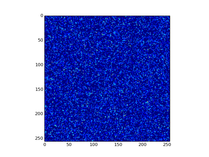
Here, as in the first example, particles2density is a function executed on the engines by pyDive.algorithm.map(). All of its arguments are numpy-arrays or structures (pyDive.arrayOfStructs) of numpy-arrays.

pyDive.algorithm.map() can also be used as a decorator:

@pyDive.map
def particles2density(particles, density):
    ...

particles2density(particles, density)

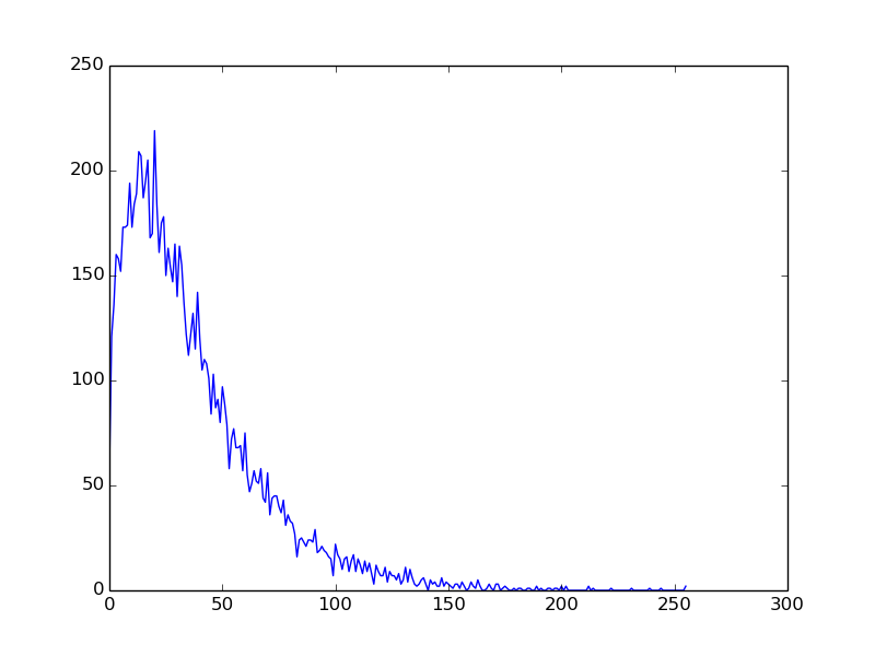
Example 3: Particle energy spectrum

import pyDive
import numpy as np
pyDive.init()

bins = 256
spectrum = pyDive.cloned.zeros([bins])

h5input = "sample.h5"

velocities = pyDive.h5.open(h5input, "/particles/vel")

@pyDive.map
def vel2spectrum(velocities, spectrum, bins):
    velocities = velocities.load()
    mass = 1.0
    energies = 0.5 * mass * (velocities.x**2 + velocities.y**2 + velocities.z**2)

    spectrum[:], bin_edges = np.histogram(energies, bins)

vel2spectrum(velocities, spectrum, bins=bins)

final_spectrum = spectrum.sum() # add up all local copies

from matplotlib import pyplot as plt
plt.plot(final_spectrum)
plt.show()

Output: